Dragonflow Deep Dive (Part 1)

In this post i am going to do a deep dive introduction to Dragonflow. Dragonflow is an embedded L3 controller in Neutron that solves the network node bottleneck the SDN way, and overcomes some of the DVR limitations. It is aligned as an Openstack Neutron L3 Plugin and provide DVR functionality without the use of namespaces or L3 agents in the compute nodes.

You can read a detailed introduction and a high level overview of the solution in here.

In this post i am going to start and show you how Dragonflow works, and how the logical flows actually translate to openflow flows inside openvswitch.

The first step i did was to install Dragonflow using the devstack plugin, you can read the full instructions here

The following diagram shows us the configured pipeline to each of the openvswitch in the setup, and i will refer to it during this explanation.

Basic Default Pipeline

Let’s first observe at the configured flows after devstack is up and analyze them, (This is done with the ‘ovs-ofctl dump-flows br-int’ command)

 1.cookie=0x0, duration=2205.752s, table=0, n_packets=0, n_bytes=0, priority=1 actions=goto_table:40
 2.cookie=0x0, duration=2205.757s, table=0, n_packets=0, n_bytes=0, priority=0 actions=NORMAL
 3.cookie=0x0, duration=2205.752s, table=0, n_packets=0, n_bytes=0, priority=1000,in_port=6 actions=NORMAL
 4.cookie=0x0, duration=2205.752s, table=0, n_packets=0, n_bytes=0, priority=1000,in_port=2 actions=NORMAL
 5.cookie=0x0, duration=2211.729s, table=23, n_packets=0, n_bytes=0, priority=0 actions=drop
 6.cookie=0x0, duration=2205.752s, table=40, n_packets=0, n_bytes=0, priority=10,dl_dst=01:00:00:00:00:00/01:00:00:00:00:00 actions=NORMAL
 7.cookie=0x0, duration=2205.752s, table=40, n_packets=0, n_bytes=0, priority=1 actions=goto_table:52
 8.cookie=0x0, duration=2205.752s, table=40, n_packets=0, n_bytes=0, priority=100,dl_dst=ff:ff:ff:ff:ff:ff actions=NORMAL
 9.cookie=0x0, duration=2205.752s, table=40, n_packets=0, n_bytes=0, priority=1000,arp actions=goto_table:51
 10.cookie=0x0, duration=2205.752s, table=51, n_packets=0, n_bytes=0, priority=1 actions=NORMAL
 11.cookie=0x0, duration=2205.752s, table=52, n_packets=0, n_bytes=0, priority=1 actions=goto_table:53
 12.cookie=0x0, duration=2211.658s, table=60, n_packets=0, n_bytes=0, priority=1 actions=move:NXM_NX_TUN_ID[0..31]->NXM_NX_PKT_MARK[],output:6

We can see in the flow list the basic pipeline install, this happen for every compute node regardless of the configuration. Its important to remember that the bigger Openflow priority number means the higher priority (the flows which are first checked for a match)

I will break the above flows into their tables and explain each one, you can see in the above pipeline diagram how this aligns with what is described there.

Table 0

Flow 1 is the default flow in the main table (‘0’), which is also the first table for every new packet entering the switch, this flow sends all traffic which is recived from a VM port to the classifier table (table 40)

Since we are in a single node setup, we can also see specific flows for the dhcp/patch-tun which output to the NORMAL path (flows 3 and 4) (for DHCP this is the port that connects br-int to the namespace where dnsmasq is running in)

Table 40

Flows 6 and 8 match any boradcast or multicast traffic (dst MAC 01:00:00:00:00:00 or ff:ff:ff:ff:ff:ff), their action is to output it to the NORMAL path. (Dragonflow doesnt handle L2 with its own flows yet, but it is planned)

Flow 9 matches any ARP packets and send them to table 51, we will see that when routers are added, Dragonflow installs ARP responders for the router ports in table 51

Default flow (flow 7), if nothing was matched before, send it to table 52 which implements our virtual distributed router

Table 51, 52 and 60

Flow 10 is the default flow in table 51 which sends the traffic to the NORMAL pipeline

Flow 11 is the default flow which sends traffic from our L3 DVR implementation table (52) to the public table (53), any traffic that matches on this flow is a north-south traffic (SNAT/DNAT), in the next posts i will show and describe how we match all the east-west traffic before defaulting to this flow. (And hence making sure that if we reach this default, this is a public external traffic)

Flow 12 in table 60 translate tunnel id to packet markup field, here is a detailed background why this is used

For each VM port attached to openvswitch, we add a flow to write the segmentation id (tunnel id) to the packet meta data field depending on the port number, this classify to which network the vm belongs. (We will see this flow installed in table ‘0’ in the next post when VM’s are added)

How ever when packets cross between OVS bridges, in our case from br-int to br-tun, this information is lost, the only saved information OVS support is in the markup field, that is why this flow is needed, to move this information to the markup field. (Metadata is standard in OF, while the markup is just used in OVS as a patch)

Another interesting thing to notice is table 23 (flow 5), this is called the CANARY TABLE and it contains a dummy flow which is added by Neutron L2 agent and is used to detect if openvswitch was restarted (when the flow is not there). The agent constantly poll and search for this flow in order to do that.

Pipeline After Configuring Two Networks and a Router

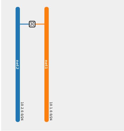
Now after we saw and understood the default pipeline, lets add two networks (net1 and net2 with subnets 10.0.1.0/24 and 10.0.2.0/24) and connect them with a router.

The following diagram shows the network topology in Openstack UI

After we finished the configuration, we can re-check the flows table, for simplicity i only paste the new added flows, all the above flows remains the same

 1.cookie=0x0, duration=3063.423s, table=0, n_packets=0, n_bytes=0, priority=1000,in_port=8 actions=NORMAL
 2.cookie=0x0, duration=3063.423s, table=0, n_packets=0, n_bytes=0, priority=1000,in_port=7 actions=NORMAL
 3.cookie=0x0, duration=3063.422s, table=51, n_packets=0, n_bytes=0, send_flow_rem priority=100,arp,metadata=0x1f42,arp_tpa=10.1.0.1,arp_op=1 actions=set_field:2->arp_op,move:NXM_NX_ARP_SHA[]->NXM_NX_ARP_THA[],move:NXM_OF_ARP_SPA[]->NXM_OF_ARP_TPA[],set_field:fa:16:3e:c0:8d:8b->eth_src,set_field:fa:16:3e:c0:8d:8b->arp_sha,set_field:10.1.0.1->arp_spa,IN_PORT
 4.cookie=0x0, duration=3063.423s, table=51, n_packets=0, n_bytes=0, send_flow_rem priority=100,arp,metadata=0x1f43,arp_tpa=10.2.0.1,arp_op=1 actions=set_field:2->arp_op,move:NXM_NX_ARP_SHA[]->NXM_NX_ARP_THA[],move:NXM_OF_ARP_SPA[]->NXM_OF_ARP_TPA[],set_field:fa:16:3e:c5:02:4d->eth_src,set_field:fa:16:3e:c5:02:4d->arp_sha,set_field:10.2.0.1->arp_spa,IN_PORT
 5.cookie=0x0, duration=3063.423s, table=52, n_packets=0, n_bytes=0, priority=20,ip,metadata=0x1f43,nw_dst=10.1.0.0/24 actions=CONTROLLER:65535
 6.cookie=0x0, duration=3063.421s, table=52, n_packets=0, n_bytes=0, priority=30,ip,metadata=0x1f42,nw_dst=10.1.0.0/24 actions=NORMAL
 7.cookie=0x0, duration=3063.423s, table=52, n_packets=0, n_bytes=0, priority=20,ip,metadata=0x1f42,nw_dst=10.2.0.0/24 actions=CONTROLLER:65535
 8.cookie=0x0, duration=3063.423s, table=52, n_packets=0, n_bytes=0, priority=30,ip,metadata=0x1f43,nw_dst=10.2.0.0/24 actions=NORMAL

Table 0

We can see that two more input ports are matched and output to the NORMAL path (flows 1,2) these are the DHCP ports, one for each of the new networks (remember we are showing a single node devstack setup)

Table 51

We can see two new flows in table 51, these are the two ARP responders for each of the networks router interfaces. These flows were configured when we connected the networks to router interfaces (Remember that every ARP request is forwarded to this table after the default pipeline is installed)

These flows match ARP requests for the router interfaces IP’s (10.1.0.1 and 10.2.0.1) for network 1 and network 2 and construct and return an ARP reply with their virtual MAC addresses

Table 52

This table implements our distributed virtual L3 router, if we look closely at the flows we can see two type of flows.

One type is matching the metadata and destination ip subnet and its action is to output the traffic to the NORMAL pipeline.

What these flows do is detect an inner network communication (L2 traffic), remember that each VM port is first marked with a metadata that indicate the network that this VM belongs to (more specifically the segmentation id of this network). The network destination field in these flows matches the local subnet (or subnets in case of more than one).

If we take flow 8 for example, it means that the network with segmentation id 0x1f43 (network 2) has the subnet 10.2.0.0/24 configured. Dragonflow output the traffic to the NORMAL pipeline, however in the future it could also handle it in its own L2 specific flows.

We see that we have two flows of this kind, one for each network.

The other type of flows can be seen in flows 5 and 7. They look the same as the other type, matching on metadata and on network destination but their action is to send the traffic to the controller (running on the network node).

These flows detect east-west traffic between networks (L3 traffic), remember that the network with segmentation id 0x1f43 had the subnet 10.2.0.0/24 (we saw that in the previous type of flows which matched L2 traffic).

if we look closely at flow 5, this flow matches segmentation_id (metadata) 0x1f43 (network 2) and the network destination 10.1.0.0/24 (network 1). This means that this flow matches any traffic going from network 2 to network 1 (L3 Traffic) and sends the first packet to the controller. (We have the other direction configured as well (flow 7) from network 1 to network 2)

The controller installs for each compute node all the possible L3 combination pairs for east-west traffic, in the next post we will see that detecting all possible east-west traffic is important in order to understand what is the north-south traffic.

Its important to understand that this is not yet optimized, we install all these flows even without any VM on the compute node. An optimization task that we have in our backlog is to only send the relevant flows to each compute node depending on the different VMs on this compute node and the networks they are attached to. (Another optimization is to only add subnets that the networks in the compute node has route to)

Summary

In this post we saw the basic default pipeline install and what happens after we add two networks and connect them with a router. All the flows in this case were installed in a proactive model, meaning as soon as the configuration is applied.

In the next post we will add two VM’s one at each network and try to ping between them, we will be able to see the reactive mode as first packet reaches the controller.

Another topic is how SNAT/DNAT works in this model, we will see that too in the next posts, so stay tuned …